How Do Activation Functions Shape the Training Dynamics
(Part I) They gate the signal, keep gradients alive, and give each neuron a reason to exist
Imagine a panel of 100 specialists listening to the same briefing. If every specialist answers every question, the discussion quickly becomes noise. Instead, each specialist has a private rule for what they care about—one listens for numbers, another for emotions, another for contradictions.
But crucially, not everyone speaks every time. A gate decides whether each specialist is allowed to talk based on how relevant the input is to them. If the signal is weak or irrelevant, they stay silent. If it's strong, they contribute fully. Activation functions are these gates, allowing the system to build diverse, specialized representations instead of everyone saying the same thing.
Why Linear Networks Collapse
Mathematically, linear algebra has a "weakness": composability. If you perform two linear operations in a row, the result is just one big linear operation.
y = W₂(W₁x + b₁) + b₂
Simplifies to: y = (W₂W₁)x + (W₂b₁ + b₂)
In plain English: Two layers behave exactly like one. No matter how many layers you stack, your "Deep" network collapses into a shallow, single-layer model. We inject a non-linear function σ after every layer—y = σ(Wx + b)—to "break" the math and prevent this collapse.
The Activation Zoo
Not all folds are created equal. Choosing the wrong function can "kill" your network or make it "deaf" to errors.
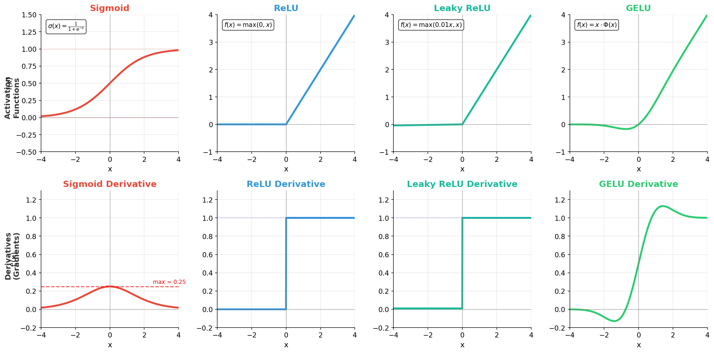
Bottom row: Their derivatives—notice Sigmoid's max gradient is only 0.25, while ReLU maintains a constant gradient of 1.0 for positive inputs.
View formulas and descriptions
| Function | Formula | Personality |
|---|---|---|
| Sigmoid | 1/(1+e⁻ˣ) | The "Squasher." Flattens everything between 0 and 1. |
| ReLU | max(0, x) | The "Gatekeeper." Fast and simple; either OFF or ON. |
| Leaky ReLU | max(0.01x, x) | The "Safety Net." Never fully turns off. |
| GELU | x·Φ(x) | The "Smooth Operator." Weights inputs by their probability. |
Experiment Setup
| Dataset | Synthetic sine wave: y = sin(x) + N(0, 0.1), x ∈ [-π, π], 200 samples |
| Architecture | 10 hidden layers × 64 neurons each (fully connected) |
| Training | 500 epochs, Adam optimizer, MSE loss |
| Activations | Sigmoid, ReLU, Leaky ReLU, GELU |
Experiment 1: The "Telephone Game" (Gradient Flow)
Training a network uses Backpropagation. Think of this as a game of "Telephone" where the error signal travels from the last layer back to the first.
The Problem: If every person in the chain whispers (multiplies the signal by a small number like 0.2), the message is gone by the time it reaches the first layer. This is the Vanishing Gradient Problem.
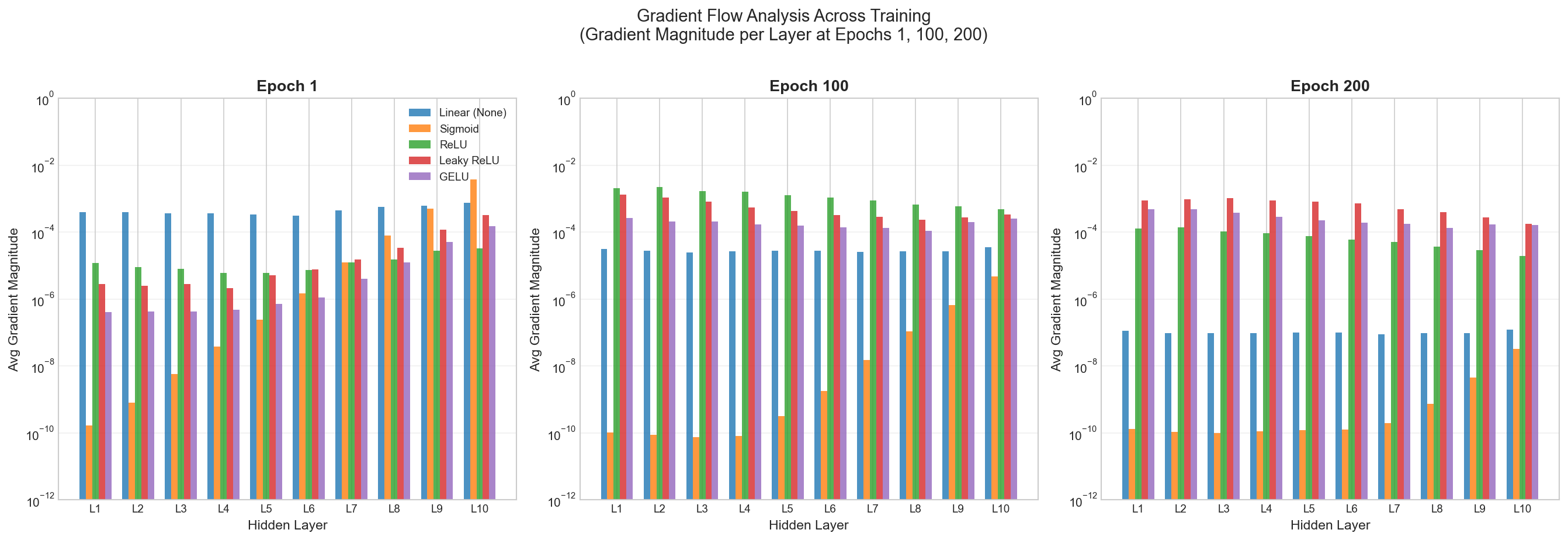
The Result: As shown in Figure 1&2, Sigmoid's maximum "volume" (derivative) is only 0.25, while ReLU's gradient is a constant 1.0 for all positive inputs. Even in a modest 10-layer network with Sigmoid, your signal becomes 0.25¹⁰ ≈ 10⁻⁶—effectively noise. The early layers learn nothing because they can't "hear" the error. ReLU, by contrast, passes the full gradient through, keeping the "telephone line" clear.
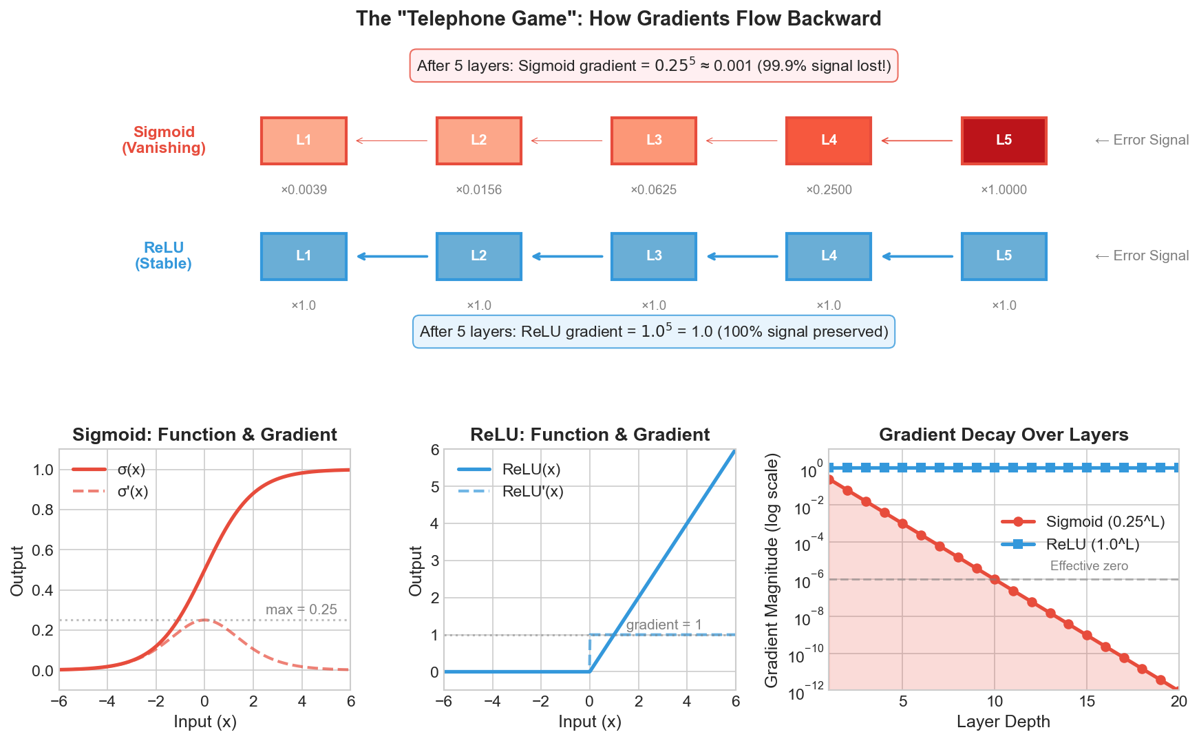
Top: The "Telephone Game" visualization showing how error signals propagate backward—Sigmoid gradients vanish exponentially while ReLU maintains full signal strength.
Bottom: Function shapes and their derivatives, and gradient magnitude decay over layers (right).
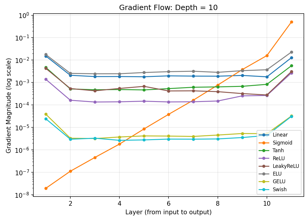
We built a 10-layer network, measured gradient magnitude at each layer during backpropagation. As shown in Figure 3, Sigmoid's gradient decays exponentially across layers while ReLU and GELU maintain stable magnitudes throughout the network.
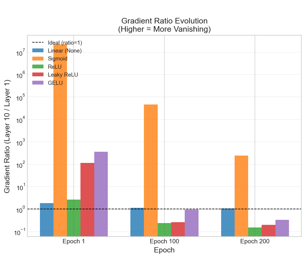
Gradient Ratio Evolution. The gradient ratio (Layer 10 / Layer 1) measures how much the error signal shrinks as it travels from the output back to the input—a ratio close to 1.0 means the gradient flows evenly, while a large ratio indicates severe vanishing. As shown in Figure 4, ReLU and GELU converge toward the ideal ratio of 1.0 over training, while Sigmoid remains orders of magnitude above.
Gradient Magnitude Over Training. We also tracked how gradient magnitudes at each layer evolve throughout training (Figure 5). Early in training, gradients are larger as the network makes big adjustments; as convergence approaches, gradients shrink. The key observation: ReLU and GELU maintain consistent layer-wise gradient patterns across epochs, while Sigmoid's early layers remain starved of signal throughout.
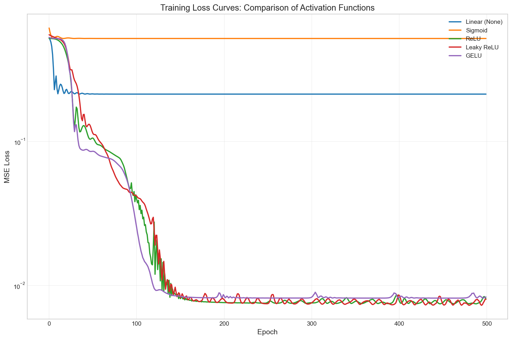
Training Loss Curves. The gradient flow directly impacts whether the network learns. Figure 6 shows the loss curves for each activation function over 500 epochs—ReLU/GELU converge quickly while Sigmoid flatlines.
Experiment 2: The "Dead Neuron" Crisis
A Dead Neuron is a light switch stuck in the "OFF" position.
In ReLU, if the input is negative, the output is 0 and the gradient (the "learning signal") is also 0. If a neuron's weights get pushed too far into the negative, it stops updating entirely. It is effectively "brain dead" for the rest of training.
Leaky ReLU adds a tiny slope to the negative side. This ensures that even if a neuron is "off," it still passes a tiny bit of signal so it can eventually "wake up" and learn again.
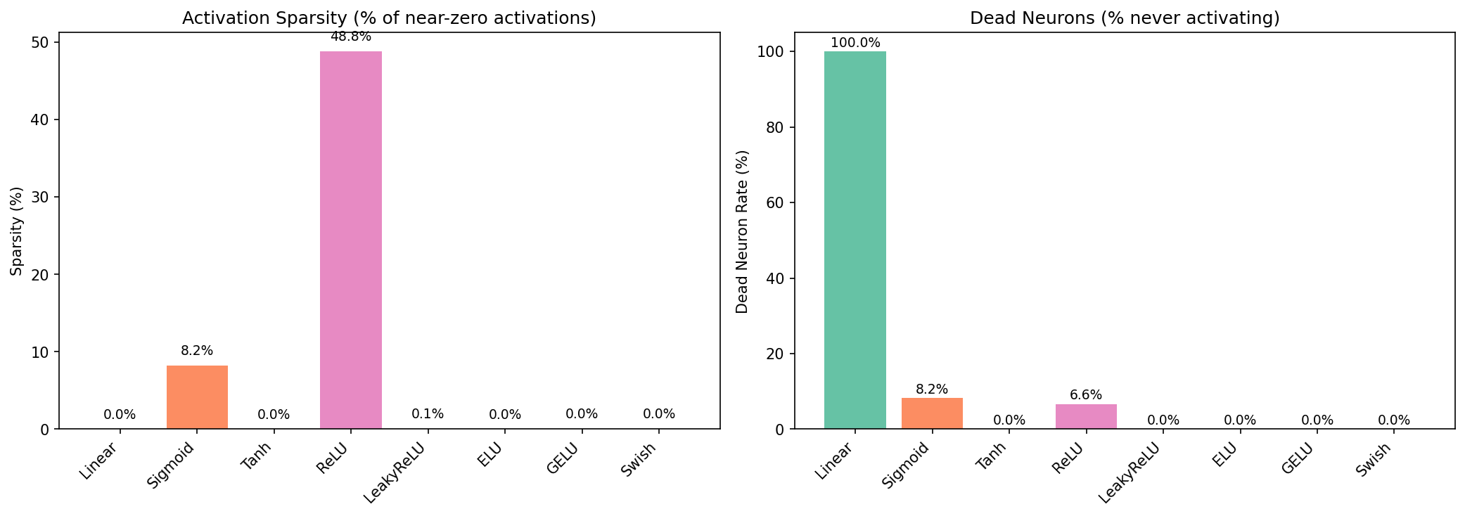
We trained 10-layer networks with a high learning rate (0.1) to stress-test each activation and measured dead neuron rate (neurons that never activate across the dataset).
More Results
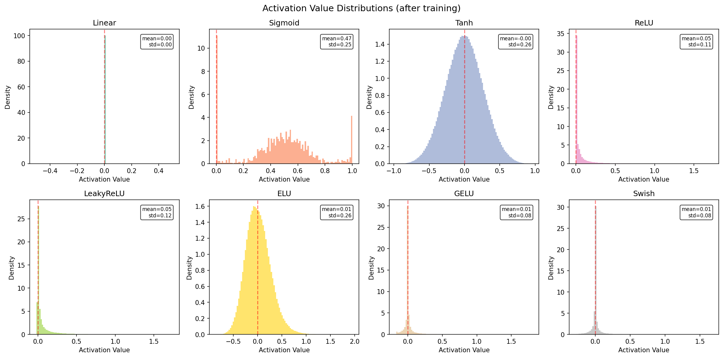
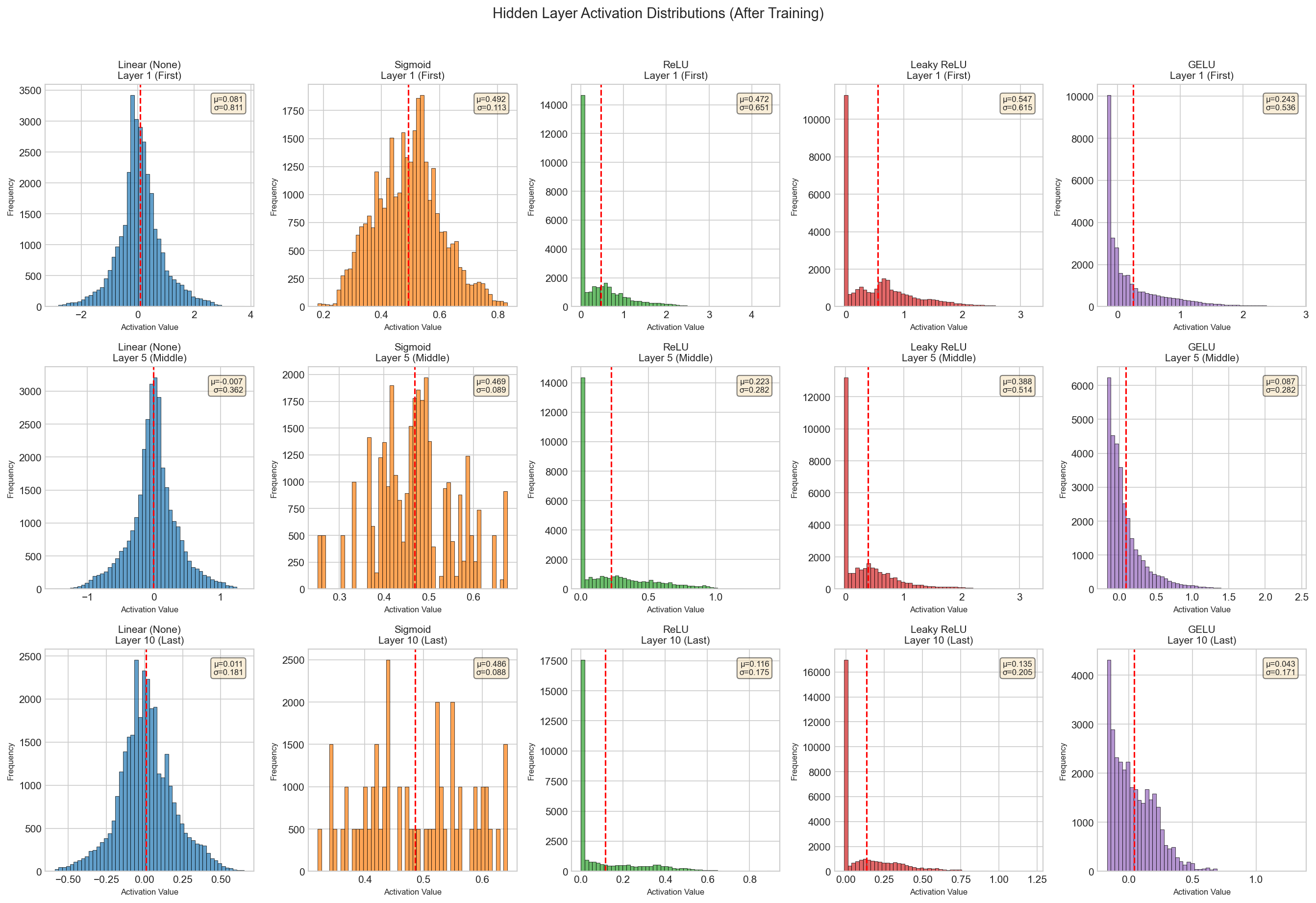
Activation Distributions. The distribution of activation values reveals how each function transforms the input signal:
Hidden Layer Activations. What do the actual activation patterns look like at different layers? Here we visualize the internal representations at layers 1, 5, and 10:
Experiment 3: Representational "Texture"
Different functions have different "personalities" that suit different data types:
- ReLU is "Jagged": It creates sharp, piecewise linear boundaries. It's excellent for rigid classification (e.g., "Is this a truck?").
- GELU is "Smooth": It curves gently. Modern architectures like Transformers prefer this because it interacts better with Layer Normalization, preventing the "starkness" of ReLU from causing training jitters.
We trained 5-layer networks for 500 epochs to approximate 5 target functions: sin(x), |x| (absolute value), step function, sin(10x) (high frequency), and x³ (polynomial).
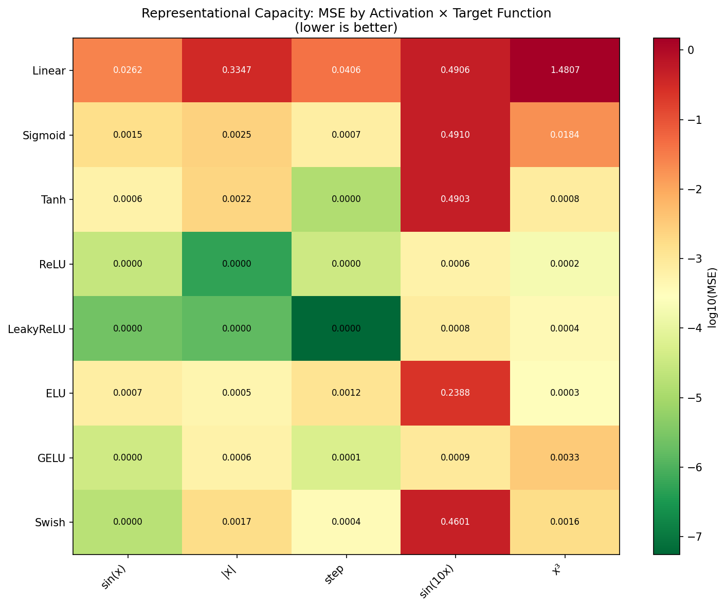
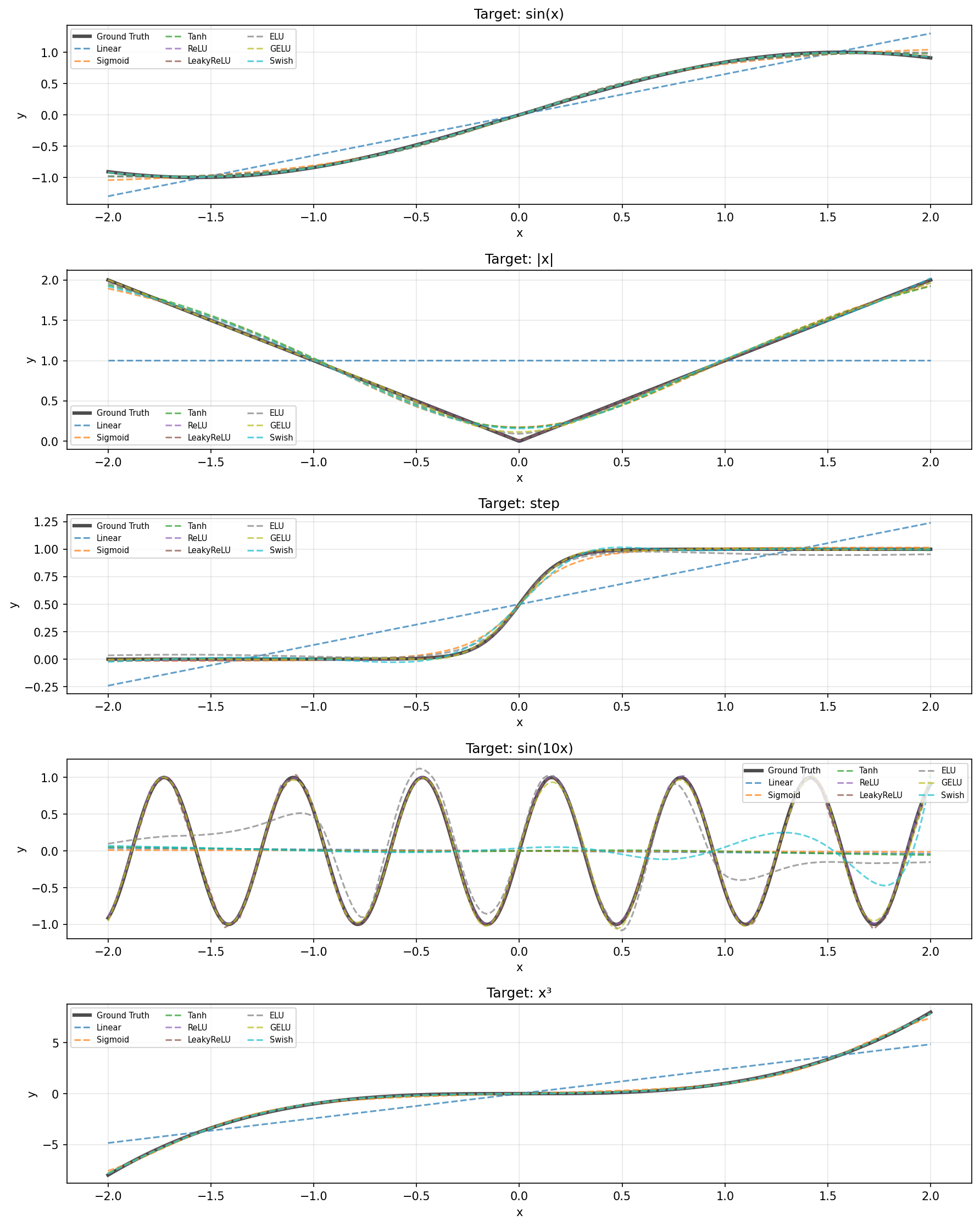
Key insight: ReLU's piecewise-linear nature makes it particularly effective at approximating sharp functions like |x|. Leaky ReLU performs best on smooth targets like sin(x), likely because its small negative slope aids optimization rather than due to smoothness matching.
Activation Functions in Frontier LLM Research
In today's frontier model training—at the scale of OpenAI and Anthropic—activation functions are no longer a minor architectural choice but a stability and efficiency primitive. The hot take is that modern activations are designed less for expressivity and more for controllable gradient flow, numerical stability, and hardware efficiency at extreme depth and width.
At scale, even small activation quirks amplify: dead neurons, saturation regions, or sharp nonlinearities can silently degrade effective model capacity, slow convergence, or destabilize long-horizon training. Functions like GELU / SiLU (Swish) dominate not because they are theoretically superior in isolation, but because their smooth, non-saturating behavior reduces gradient pathologies across hundreds of layers, interacts favorably with LayerNorm and residual streams, and remains robust under mixed precision and large batch training. While GELU is more computationally expensive than ReLU (requiring error functions or sigmoids), modern GPUs handle these transcendental functions with near-zero latency penalty via specialized hardware units—the real "efficiency" is convergence efficiency: reaching lower loss in fewer steps.
Experiments and post generated with Orchestra.