Why Deep Networks Need Residual Connections
A controlled experiment on the vanishing gradient problem
Imagine you're playing a game of Telephone with 100 people. You whisper "The sky is blue" to the first person. By the time it reaches the 20th person, it's a faint mumble. By the 100th? Total silence.
This is exactly what happens inside deep neural networks — and for decades, it was an unsolved problem that blocked progress in AI.
The Mystery: The Dead Layers
When we train a neural network, information flows in two directions. Forward: data passes through layers to make a prediction. Backward: gradients flow back to tell each layer how to improve.
The problem? In a deep network, these backward-flowing gradients get multiplied by small numbers at every layer:
Layer 20: "Hey, adjust your weights by 0.01!"
Layer 10: "Adjust by 0.000001..."
Layer 1: 10-19 (essentially zero)
The early layers — the very foundation of the network — receive no learning signal. They are frozen in time, while only the last few layers do any meaningful work. This is the vanishing gradient problem.
The Experiment: Can You Pass the Ball?
To prove how severe this problem is, we designed the simplest possible test. We asked two 20-layer networks one question: Can you just pass the input X to the output Y without breaking it?
This is the "Distant Identity" task (Y = X). If a network can't even learn to do nothing, it certainly can't learn anything useful. And we compared two architectures, identical except for one line of code:
PlainMLP (The Old Way)
x = ReLU(Linear(x))
Standard feedforward. Each layer transforms the input completely.
Philosophy: "Transform everything."
ResMLP (The Residual Way)
x = x + ReLU(Linear(x))
Residual connection. The input is added back to the output.
Philosophy: "Keep what you have, then add to it."
Both models use identical initialization: Kaiming He weights scaled by 1/√20, zero biases, no normalization layers. The only difference is the + x residual connection.
| Depth | 20 layers |
| Hidden dim | 64 |
| Optimizer | Adam (lr=1e-3) |
| Steps | 500 |
| Batch size | 64 |
The Results: Total Collapse vs. Total Success
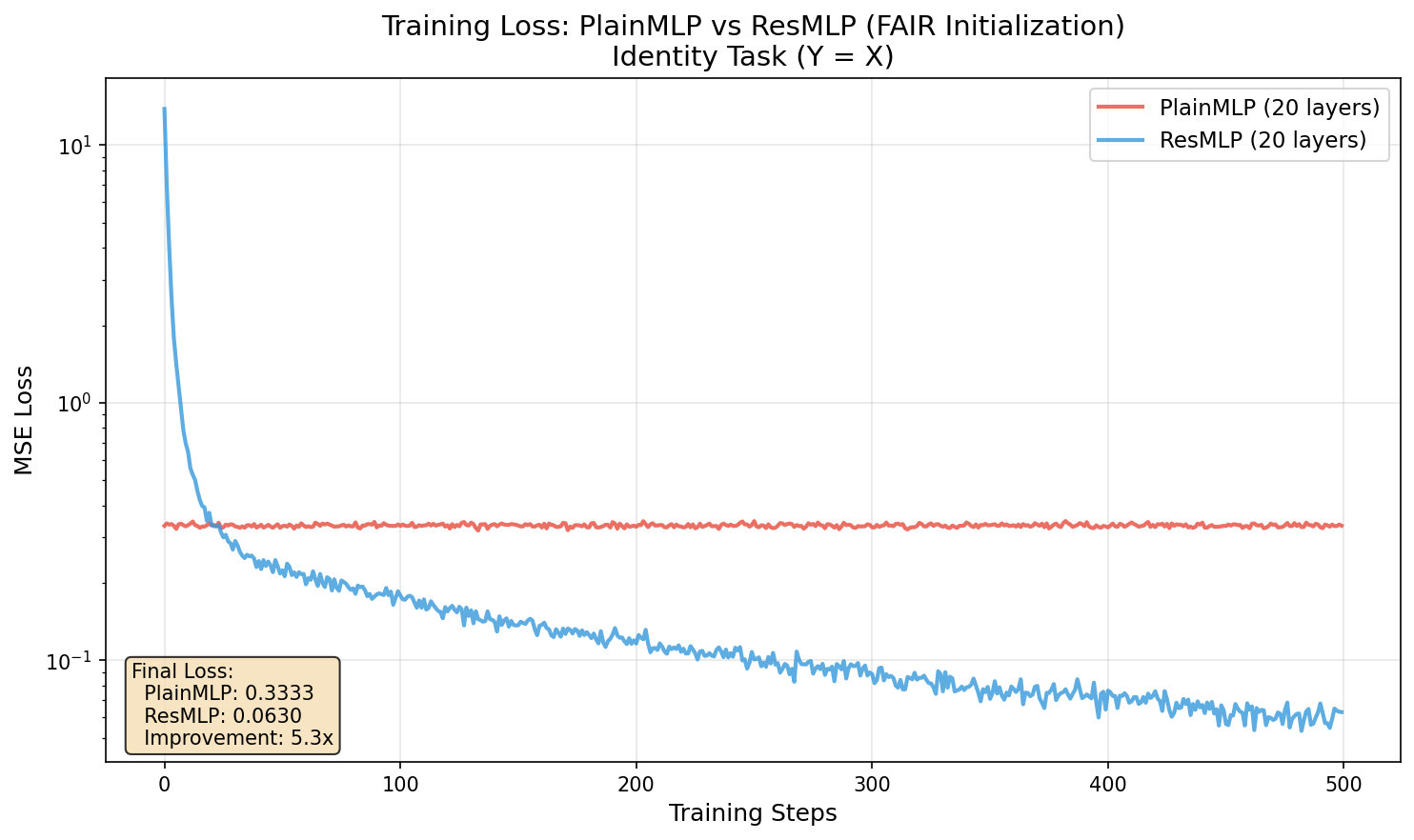
The PlainMLP failed the test completely. It couldn't even learn to do nothing. Starting at loss 0.333, it ended at... 0.333. Zero improvement.
Meanwhile, ResMLP started at a higher loss (13.8, because the residual branches add noise initially) but dropped to 0.063 — a 99.5% reduction. The residual network learns; the plain network is completely stuck.
| Metric | PlainMLP | ResMLP |
|---|---|---|
| Initial Loss | 0.333 | 13.826 |
| Final Loss | 0.333 | 0.063 |
| Loss Reduction | 0% | 99.5% |
The Diagnosis: Why the Plain Network Died
We looked under the hood to see why the PlainMLP failed. Two things happened:
Forward Signal Collapse
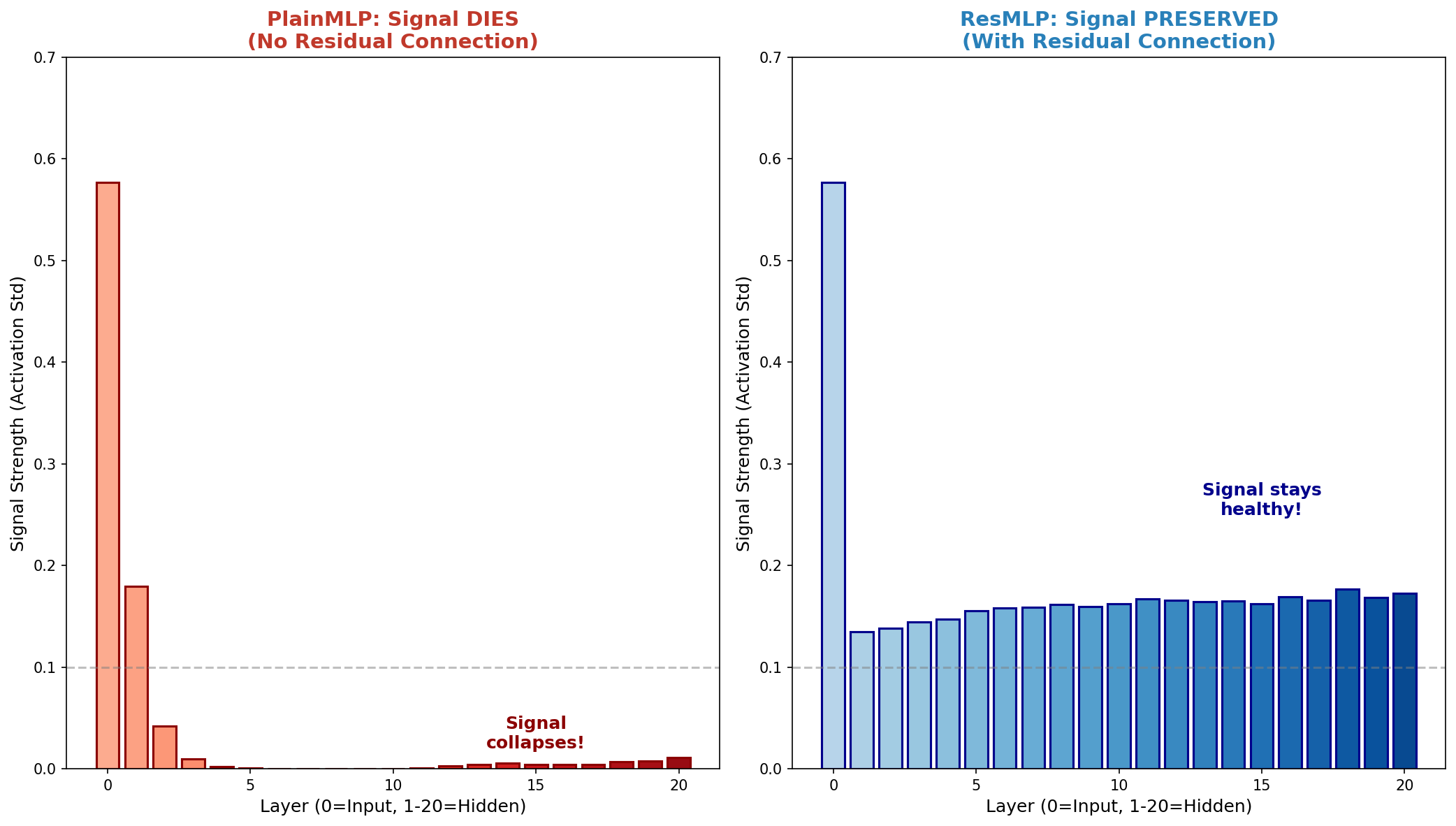
In PlainMLP, the signal strength starts healthy but collapses to near-zero by layer 5. Every time data passes through a ReLU activation, approximately 50% is deleted (all negatives become 0). The decay is exponential — by layer 20, the network has literally "forgotten" what the input looked like.
In ResMLP, the + x ensures the original signal is always added back, keeping activations stable around 0.13-0.18 throughout all 20 layers.
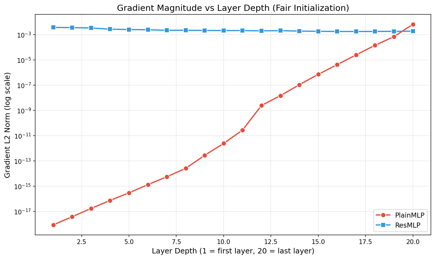
Backward Gradient Vanishing
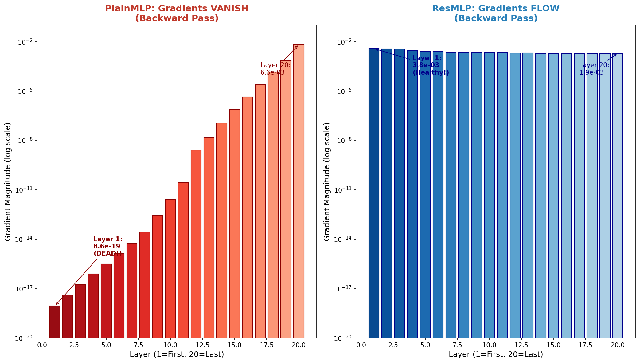
The gradient situation is even more dramatic. In PlainMLP, the gradient at layer 20 is ~10-3, but by layer 1 it's 8.6 × 10⁻¹⁹ — essentially zero. That's a decay of 16 orders of magnitude across just 20 layers.
In ResMLP, gradients stay healthy at ~10-3 across all layers. Early layers receive a real learning signal and can actually update their weights.
Intuition Check
If the gradient at the output layer is a gallon of water, by the time it reaches layer 1 in a PlainMLP, it's less than a single atom. You can't wash a car with an atom of water — and you can't train a layer with 10-19 gradient.
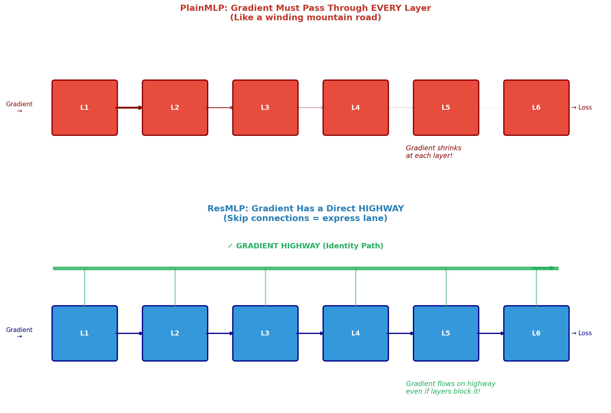
The Solution: The Gradient Highway
In 2015, Kaiming He and his team at Microsoft Research introduced a beautifully simple fix: the residual connection. It acts like an express lane on a crowded highway.
Instead of forcing gradients to pass through every layer (a winding mountain road), the skip connection creates a direct highway that bypasses the transformations entirely.
The Math of the "Plus One"
The secret lies in calculus. The chain rule explains why gradients vanish — and why residuals fix it:
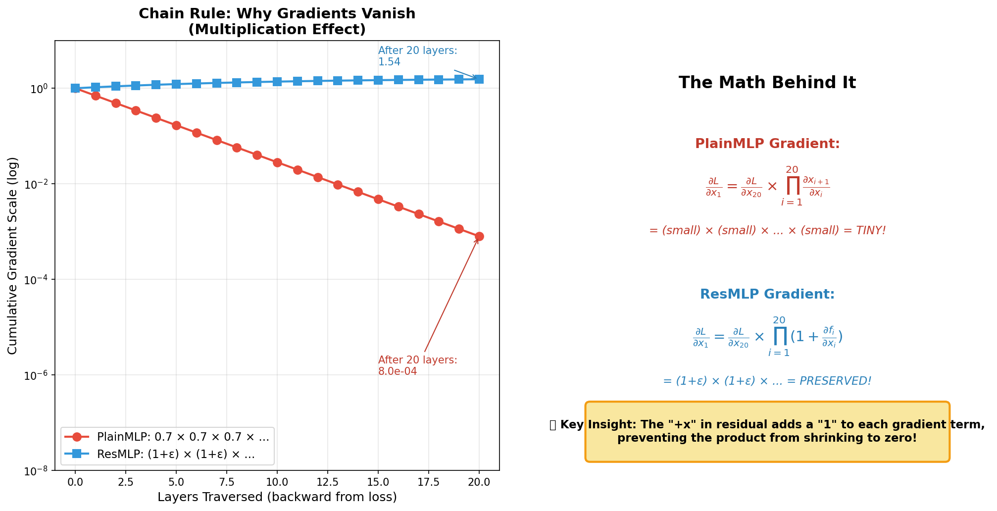
Without Residual: x = f(x)
∂xn/∂x1 = ∏ (∂f/∂x)i
Each term < 1, so the product → 0 as layers increase.
With Residual: x = x + f(x)
∂xn/∂x1 = ∏ (1 + ∂f/∂x)i
The "+1" ensures each term ≥ 1, so the product never vanishes.
This single insight — adding a "1" to each gradient term — is what enables training networks with 100+ layers.
Activation Statistics
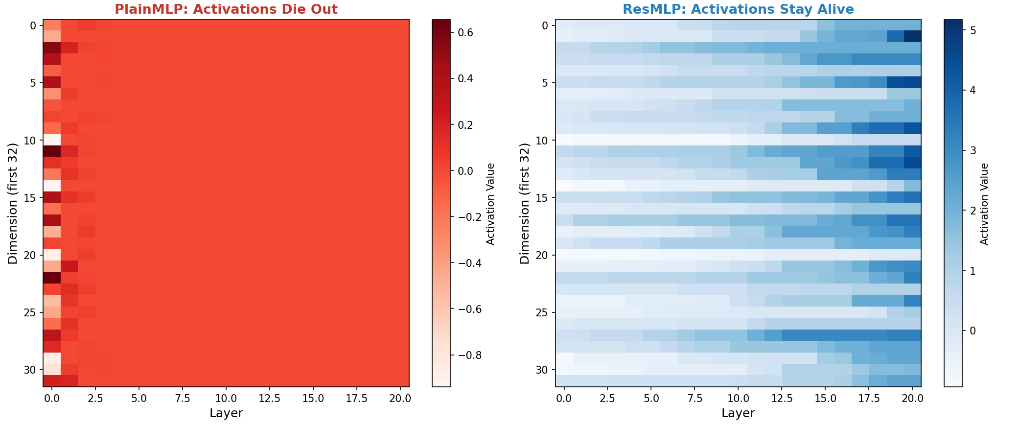
Left: PlainMLP activations die out after layer 2, collapsing to near-zero (red).
Right: ResMLP activations stay alive throughout all layers (blue gradient).
Residual Connections in Frontier LLM Research
The residual connection x = x + f(x) does one simple but profound thing: it ensures the gradient can never shrink to zero. This matters most for deep networks — the deeper the model, the more layers gradients must traverse, and the more critical that "gradient highway" becomes.
Why does this matter for frontier LLMs? Large models like LLaMA-70B stack 80 transformer layers, and GPT-3 uses 96. As models grow deeper and wider, residual connections have evolved into more than just "x + f(x)." Frontier architectures now use gated residuals [1], scaled residuals (e.g., multiplying residual branches by a learned or fixed α) [2], residual stream scaling [3], and parallel residual streams [4]. These tweaks control gradient flow, reduce training instability, and prevent any single layer from dominating the signal.
References:
[1] Dynamic Context Adaptation and Information Flow Control in Transformers
[2] M2R2: Mixture of Multi-Rate Residuals for Efficient Transformer Inference
[3] Residual Matrix Transformers: Scaling the Size of the Residual Stream
Experiments and post generated with Orchestra.